Note

Go to the end to download the full example code or to run this example in your browser via JupyterLite or Binder

Comparison of the K-Means and MiniBatchKMeans clustering algorithms#

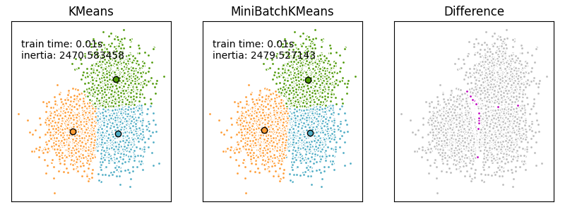
We want to compare the performance of the MiniBatchKMeans and KMeans: the MiniBatchKMeans is faster, but gives slightly different results (see Mini Batch K-Means).

We will cluster a set of data, first with KMeans and then with MiniBatchKMeans, and plot the results. We will also plot the points that are labelled differently between the two algorithms.

Generate the data#

We start by generating the blobs of data to be clustered.

import numpy as np

from sklearn.datasets import make_blobs

np.random.seed(0)

batch_size = 45
centers = [[1, 1], [-1, -1], [1, -1]]
n_clusters = len(centers)
X, labels_true = make_blobs(n_samples=3000, centers=centers, cluster_std=0.7)

Compute clustering with KMeans#

import time

from sklearn.cluster import KMeans

k_means = KMeans(init="k-means++", n_clusters=3, n_init=10)
t0 = time.time()
k_means.fit(X)
t_batch = time.time() - t0

Compute clustering with MiniBatchKMeans#

from sklearn.cluster import MiniBatchKMeans

mbk = MiniBatchKMeans(
    init="k-means++",
    n_clusters=3,
    batch_size=batch_size,
    n_init=10,
    max_no_improvement=10,
    verbose=0,
)
t0 = time.time()
mbk.fit(X)
t_mini_batch = time.time() - t0

Establishing parity between clusters#

We want to have the same color for the same cluster from both the MiniBatchKMeans and the KMeans algorithm. Let’s pair the cluster centers per closest one.

from sklearn.metrics.pairwise import pairwise_distances_argmin

k_means_cluster_centers = k_means.cluster_centers_
order = pairwise_distances_argmin(k_means.cluster_centers_, mbk.cluster_centers_)
mbk_means_cluster_centers = mbk.cluster_centers_[order]

k_means_labels = pairwise_distances_argmin(X, k_means_cluster_centers)
mbk_means_labels = pairwise_distances_argmin(X, mbk_means_cluster_centers)

Plotting the results#

import matplotlib.pyplot as plt

fig = plt.figure(figsize=(8, 3))
fig.subplots_adjust(left=0.02, right=0.98, bottom=0.05, top=0.9)
colors = ["#4EACC5", "#FF9C34", "#4E9A06"]

# KMeans
ax = fig.add_subplot(1, 3, 1)
for k, col in zip(range(n_clusters), colors):
    my_members = k_means_labels == k
    cluster_center = k_means_cluster_centers[k]
    ax.plot(X[my_members, 0], X[my_members, 1], "w", markerfacecolor=col, marker=".")
    ax.plot(
        cluster_center[0],
        cluster_center[1],
        "o",
        markerfacecolor=col,
        markeredgecolor="k",
        markersize=6,
    )
ax.set_title("KMeans")
ax.set_xticks(())
ax.set_yticks(())
plt.text(-3.5, 1.8, "train time: %.2fs\ninertia: %f" % (t_batch, k_means.inertia_))

# MiniBatchKMeans
ax = fig.add_subplot(1, 3, 2)
for k, col in zip(range(n_clusters), colors):
    my_members = mbk_means_labels == k
    cluster_center = mbk_means_cluster_centers[k]
    ax.plot(X[my_members, 0], X[my_members, 1], "w", markerfacecolor=col, marker=".")
    ax.plot(
        cluster_center[0],
        cluster_center[1],
        "o",
        markerfacecolor=col,
        markeredgecolor="k",
        markersize=6,
    )
ax.set_title("MiniBatchKMeans")
ax.set_xticks(())
ax.set_yticks(())
plt.text(-3.5, 1.8, "train time: %.2fs\ninertia: %f" % (t_mini_batch, mbk.inertia_))

# Initialize the different array to all False
different = mbk_means_labels == 4
ax = fig.add_subplot(1, 3, 3)

for k in range(n_clusters):
    different += (k_means_labels == k) != (mbk_means_labels == k)

identical = np.logical_not(different)
ax.plot(X[identical, 0], X[identical, 1], "w", markerfacecolor="#bbbbbb", marker=".")
ax.plot(X[different, 0], X[different, 1], "w", markerfacecolor="m", marker=".")
ax.set_title("Difference")
ax.set_xticks(())
ax.set_yticks(())

plt.show()