sklearn.mixture.GaussianMixture#
- class sklearn.mixture.GaussianMixture(n_components=1, *, covariance_type='full', tol=0.001, reg_covar=1e-06, max_iter=100, n_init=1, init_params='kmeans', weights_init=None, means_init=None, precisions_init=None, random_state=None, warm_start=False, verbose=0, verbose_interval=10)[source]#
Gaussian Mixture.
Representation of a Gaussian mixture model probability distribution. This class allows to estimate the parameters of a Gaussian mixture distribution.
Read more in the User Guide.
New in version 0.18.
- Parameters:
- n_componentsint, default=1
The number of mixture components.
- covariance_type{‘full’, ‘tied’, ‘diag’, ‘spherical’}, default=’full’
String describing the type of covariance parameters to use. Must be one of:
‘full’: each component has its own general covariance matrix.
‘tied’: all components share the same general covariance matrix.
‘diag’: each component has its own diagonal covariance matrix.
‘spherical’: each component has its own single variance.
- tolfloat, default=1e-3
The convergence threshold. EM iterations will stop when the lower bound average gain is below this threshold.
- reg_covarfloat, default=1e-6
Non-negative regularization added to the diagonal of covariance. Allows to assure that the covariance matrices are all positive.
- max_iterint, default=100
The number of EM iterations to perform.
- n_initint, default=1
The number of initializations to perform. The best results are kept.
- init_params{‘kmeans’, ‘k-means++’, ‘random’, ‘random_from_data’}, default=’kmeans’
The method used to initialize the weights, the means and the precisions. String must be one of:
‘kmeans’ : responsibilities are initialized using kmeans.
‘k-means++’ : use the k-means++ method to initialize.
‘random’ : responsibilities are initialized randomly.
‘random_from_data’ : initial means are randomly selected data points.
Changed in version v1.1:
init_paramsnow accepts ‘random_from_data’ and ‘k-means++’ as initialization methods.- weights_initarray-like of shape (n_components, ), default=None
The user-provided initial weights. If it is None, weights are initialized using the
init_paramsmethod.- means_initarray-like of shape (n_components, n_features), default=None
The user-provided initial means, If it is None, means are initialized using the
init_paramsmethod.- precisions_initarray-like, default=None
The user-provided initial precisions (inverse of the covariance matrices). If it is None, precisions are initialized using the ‘init_params’ method. The shape depends on ‘covariance_type’:
(n_components,)                        if 'spherical',
(n_features, n_features)               if 'tied',
(n_components, n_features)             if 'diag',
(n_components, n_features, n_features) if 'full'
- random_stateint, RandomState instance or None, default=None
Controls the random seed given to the method chosen to initialize the parameters (see
init_params). In addition, it controls the generation of random samples from the fitted distribution (see the methodsample). Pass an int for reproducible output across multiple function calls. See Glossary.- warm_startbool, default=False
If ‘warm_start’ is True, the solution of the last fitting is used as initialization for the next call of fit(). This can speed up convergence when fit is called several times on similar problems. In that case, ‘n_init’ is ignored and only a single initialization occurs upon the first call. See the Glossary.
- verboseint, default=0
Enable verbose output. If 1 then it prints the current initialization and each iteration step. If greater than 1 then it prints also the log probability and the time needed for each step.
- verbose_intervalint, default=10
Number of iteration done before the next print.
- Attributes:
- weights_array-like of shape (n_components,)
The weights of each mixture components.
- means_array-like of shape (n_components, n_features)
The mean of each mixture component.
- covariances_array-like
The covariance of each mixture component. The shape depends on
covariance_type:(n_components,) if 'spherical', (n_features, n_features) if 'tied', (n_components, n_features) if 'diag', (n_components, n_features, n_features) if 'full'
- precisions_array-like
The precision matrices for each component in the mixture. A precision matrix is the inverse of a covariance matrix. A covariance matrix is symmetric positive definite so the mixture of Gaussian can be equivalently parameterized by the precision matrices. Storing the precision matrices instead of the covariance matrices makes it more efficient to compute the log-likelihood of new samples at test time. The shape depends on
covariance_type:(n_components,) if 'spherical', (n_features, n_features) if 'tied', (n_components, n_features) if 'diag', (n_components, n_features, n_features) if 'full'
- precisions_cholesky_array-like
The cholesky decomposition of the precision matrices of each mixture component. A precision matrix is the inverse of a covariance matrix. A covariance matrix is symmetric positive definite so the mixture of Gaussian can be equivalently parameterized by the precision matrices. Storing the precision matrices instead of the covariance matrices makes it more efficient to compute the log-likelihood of new samples at test time. The shape depends on
covariance_type:(n_components,) if 'spherical', (n_features, n_features) if 'tied', (n_components, n_features) if 'diag', (n_components, n_features, n_features) if 'full'
- converged_bool
True when convergence was reached in fit(), False otherwise.
- n_iter_int
Number of step used by the best fit of EM to reach the convergence.
- lower_bound_float
Lower bound value on the log-likelihood (of the training data with respect to the model) of the best fit of EM.
- n_features_in_int
Number of features seen during fit.
New in version 0.24.
- feature_names_in_ndarray of shape (
n_features_in_,) Names of features seen during fit. Defined only when
Xhas feature names that are all strings.New in version 1.0.
See also
BayesianGaussianMixtureGaussian mixture model fit with a variational inference.
Examples
>>> import numpy as np
>>> from sklearn.mixture import GaussianMixture
>>> X = np.array([[1, 2], [1, 4], [1, 0], [10, 2], [10, 4], [10, 0]])
>>> gm = GaussianMixture(n_components=2, random_state=0).fit(X)
>>> gm.means_
array([[10.,  2.],
       [ 1.,  2.]])
>>> gm.predict([[0, 0], [12, 3]])
array([1, 0])
Methods
aic(X)Akaike information criterion for the current model on the input X.
bic(X)Bayesian information criterion for the current model on the input X.
fit(X[, y])Estimate model parameters with the EM algorithm.
fit_predict(X[, y])Estimate model parameters using X and predict the labels for X.
Get metadata routing of this object.
get_params([deep])Get parameters for this estimator.
predict(X)Predict the labels for the data samples in X using trained model.
Evaluate the components' density for each sample.
sample([n_samples])Generate random samples from the fitted Gaussian distribution.
score(X[, y])Compute the per-sample average log-likelihood of the given data X.
Compute the log-likelihood of each sample.
set_params(**params)Set the parameters of this estimator.
- aic(X)[source]#
Akaike information criterion for the current model on the input X.
You can refer to this mathematical section for more details regarding the formulation of the AIC used.
- Parameters:
- Xarray of shape (n_samples, n_dimensions)
The input samples.
- Returns:
- aicfloat
The lower the better.
- bic(X)[source]#
Bayesian information criterion for the current model on the input X.
You can refer to this mathematical section for more details regarding the formulation of the BIC used.
- Parameters:
- Xarray of shape (n_samples, n_dimensions)
The input samples.
- Returns:
- bicfloat
The lower the better.
- fit(X, y=None)[source]#
Estimate model parameters with the EM algorithm.
The method fits the model
n_inittimes and sets the parameters with which the model has the largest likelihood or lower bound. Within each trial, the method iterates between E-step and M-step formax_itertimes until the change of likelihood or lower bound is less thantol, otherwise, aConvergenceWarningis raised. Ifwarm_startisTrue, thenn_initis ignored and a single initialization is performed upon the first call. Upon consecutive calls, training starts where it left off.- Parameters:
- Xarray-like of shape (n_samples, n_features)
List of n_features-dimensional data points. Each row corresponds to a single data point.
- yIgnored
Not used, present for API consistency by convention.
- Returns:
- selfobject
The fitted mixture.
- fit_predict(X, y=None)[source]#
Estimate model parameters using X and predict the labels for X.
The method fits the model n_init times and sets the parameters with which the model has the largest likelihood or lower bound. Within each trial, the method iterates between E-step and M-step for
max_itertimes until the change of likelihood or lower bound is less thantol, otherwise, aConvergenceWarningis raised. After fitting, it predicts the most probable label for the input data points.New in version 0.20.
- Parameters:
- Xarray-like of shape (n_samples, n_features)
List of n_features-dimensional data points. Each row corresponds to a single data point.
- yIgnored
Not used, present for API consistency by convention.
- Returns:
- labelsarray, shape (n_samples,)
Component labels.
- get_metadata_routing()[source]#
Get metadata routing of this object.
Please check User Guide on how the routing mechanism works.
- Returns:
- routingMetadataRequest
A
MetadataRequestencapsulating routing information.
- get_params(deep=True)[source]#
Get parameters for this estimator.
- Parameters:
- deepbool, default=True
If True, will return the parameters for this estimator and contained subobjects that are estimators.
- Returns:
- paramsdict
Parameter names mapped to their values.
- predict(X)[source]#
Predict the labels for the data samples in X using trained model.
- Parameters:
- Xarray-like of shape (n_samples, n_features)
List of n_features-dimensional data points. Each row corresponds to a single data point.
- Returns:
- labelsarray, shape (n_samples,)
Component labels.
- predict_proba(X)[source]#
Evaluate the components’ density for each sample.
- Parameters:
- Xarray-like of shape (n_samples, n_features)
List of n_features-dimensional data points. Each row corresponds to a single data point.
- Returns:
- resparray, shape (n_samples, n_components)
Density of each Gaussian component for each sample in X.
- sample(n_samples=1)[source]#
Generate random samples from the fitted Gaussian distribution.
- Parameters:
- n_samplesint, default=1
Number of samples to generate.
- Returns:
- Xarray, shape (n_samples, n_features)
Randomly generated sample.
- yarray, shape (nsamples,)
Component labels.
- score(X, y=None)[source]#
Compute the per-sample average log-likelihood of the given data X.
- Parameters:
- Xarray-like of shape (n_samples, n_dimensions)
List of n_features-dimensional data points. Each row corresponds to a single data point.
- yIgnored
Not used, present for API consistency by convention.
- Returns:
- log_likelihoodfloat
Log-likelihood of
Xunder the Gaussian mixture model.
- score_samples(X)[source]#
Compute the log-likelihood of each sample.
- Parameters:
- Xarray-like of shape (n_samples, n_features)
List of n_features-dimensional data points. Each row corresponds to a single data point.
- Returns:
- log_probarray, shape (n_samples,)
Log-likelihood of each sample in
Xunder the current model.
- set_params(**params)[source]#
Set the parameters of this estimator.
The method works on simple estimators as well as on nested objects (such as
Pipeline). The latter have parameters of the form<component>__<parameter>so that it’s possible to update each component of a nested object.- Parameters:
- **paramsdict
Estimator parameters.
- Returns:
- selfestimator instance
Estimator instance.
Examples using sklearn.mixture.GaussianMixture#
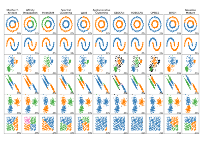
Comparing different clustering algorithms on toy datasets

